OrthoFlo
OrthoFlo is a CFD solver utilising the structured orthogonal meshing approach. Whilst this approach may introduce some limitations with respect to the complexity of the geometry that can be modelled, this approach can provide useful indicative results for some applications and may highlight whether a more comprehensive
analysis using a more advanced CFD code is necessary.
The first generation of the OrthoFlo code was written by Steve Howell of
Abercus, during his PhD studies at the University of Newcastle in 1998. Since
then, OrthoFlo has been developed through a second generation, captured in the
images below. Abercus is currently developing the third generation of the
OrthoFlo platform, which will benefit from the meshing capabilities more
recently developed as part of the OrthoMesh tool.
Second generation platform
Mesh creation
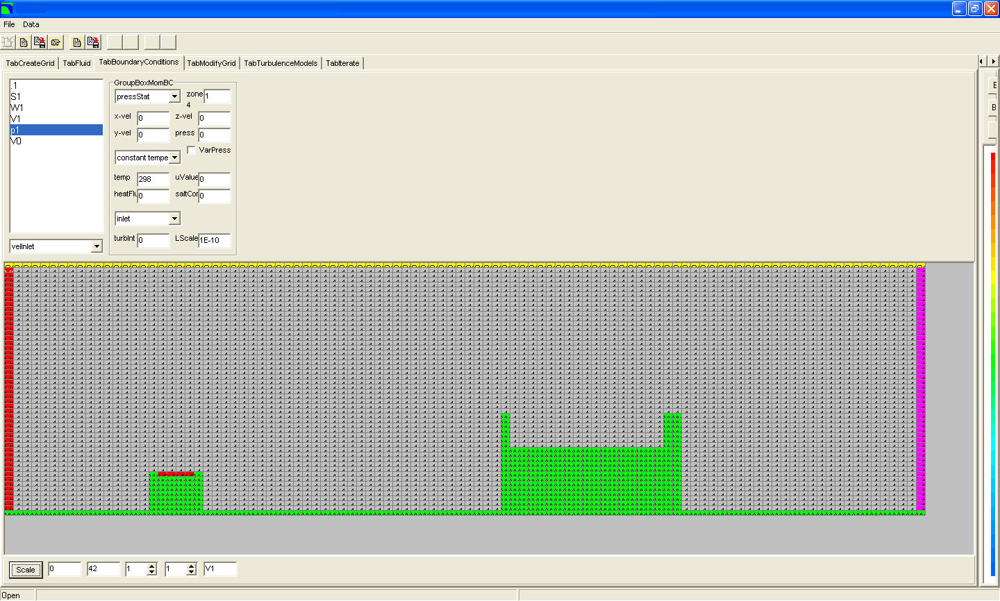
Within the second generation platform, the computational mesh is manipulated by
selecting a boundary condition and then simply dragging over a rectangular array
of cells in the grid window, across which the boundary condition will be applied
- this interface was designed to mimic that of FLUENT 4, which was in widespread
use until the late nineties.
The image below shows the mesh for a two-dimensional atmospheric dispersion
example - whilst OrthoFlo is a three-dimensional CFD code, the two-dimensional
example shown is created by taking a 2D slice of the geometry and sandwiching it
between two symmetry planes.
The green cells are solid wall boundaries - the group of cells on the left represent
an exhaust stack and the group on the right represent some obstruction downstream,
whilst the lower edge represent the ground.
The red cells are velocity inlet boundaries - those on the left represent the incoming
wind flow, and those along the top of the exhaust stack represent the hot exhaust gas.
The yellow cells along the upper edge are symmetry cells, representing a slip condition for the sky.
The magenta cells along the right hand edge are static pressure cells, and allow the
flow to escape at the leeward extent of the model.
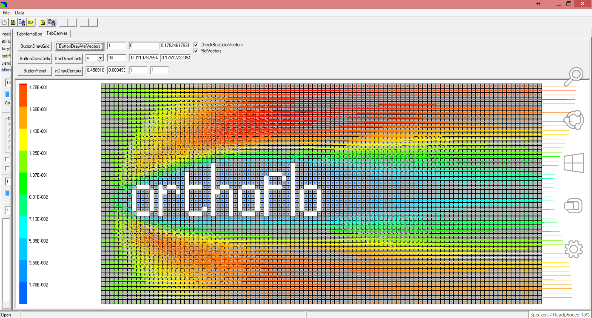
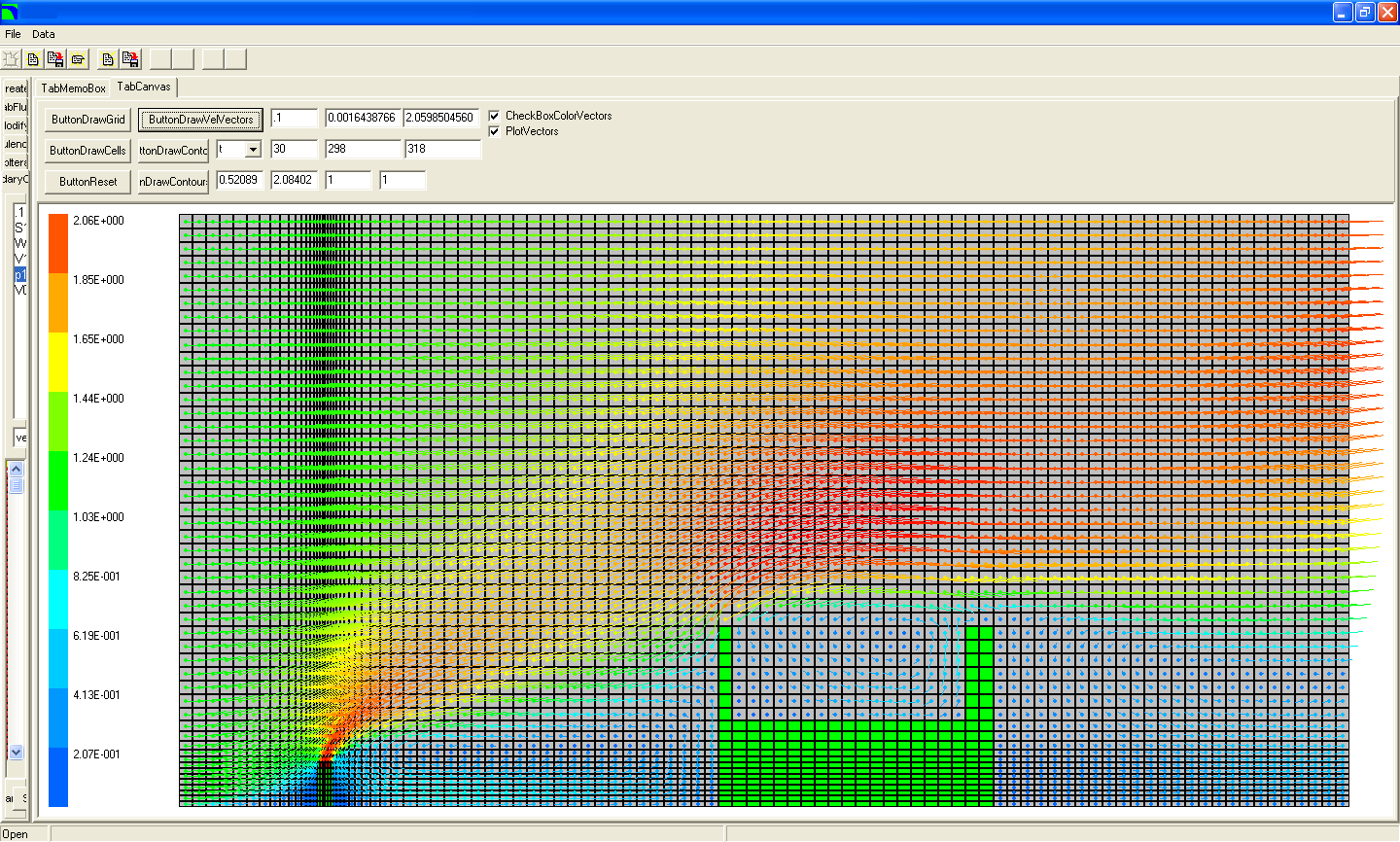
Vector plots
The velocity plot below shows the velocity vector predicted at each cell, coloured by local velocity magnitude.
The vector plot is superimposed over a plot of the geometrical grid. Notice that although mesh is necesarily
structured and orthogonal, it need not uniform - the image below shows the mesh refined in the regions of interest
around the exhaust stack.
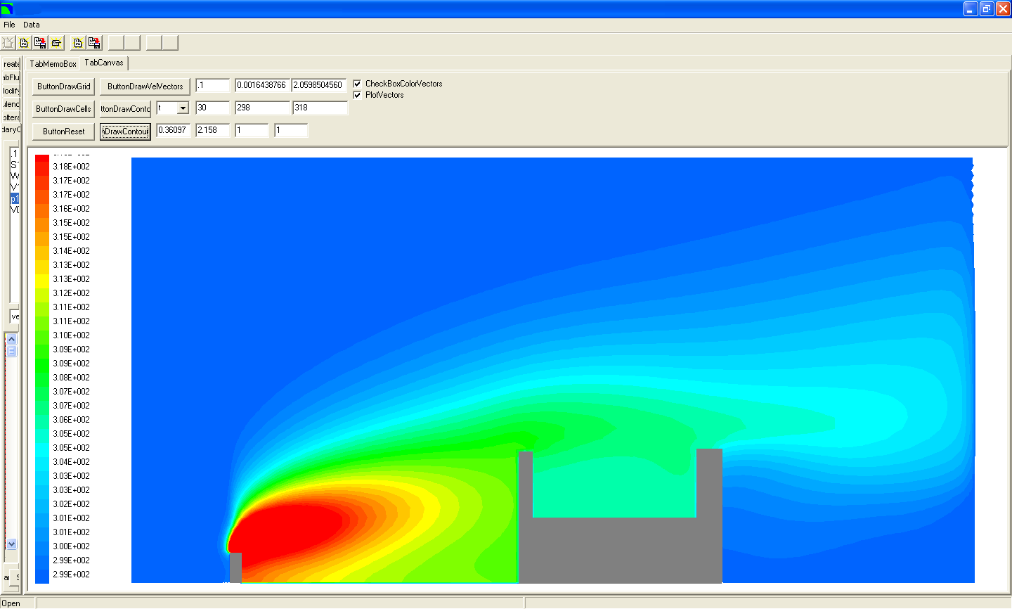
Contour plots
The contour plot below shows the dispersion pattern of the exhaust plume as it disperses over the obstruction further downstream.
The plot shows the plume to be drawn-down in the near wake of the exhaust stack
- this effect is particularly noticable for this two-dimensional example.